
Email us
![]()
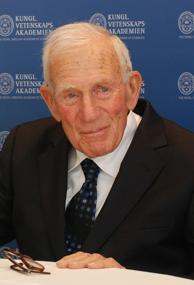
On the recent passing of the “Einstein of the Ocean”, Dr. Walter Munk, taken with permission from [1]
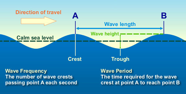
A diagram of an ocean wave showing its features, taken with permission from [4]
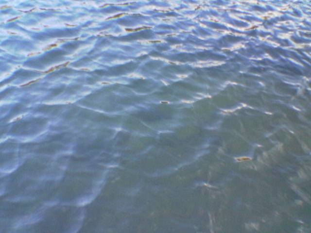
The random nature of the ocean surface, taken with permission from [5]
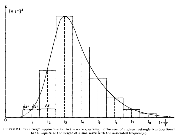
The distribution of wave lengths or frequencies in a fully-developed sea, taken with permission from [6]
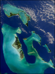
The colour of Earth’s oceans and how they might be intensified by climate change, taken with permission from [7]
A Brief History of Wavy Ocean Surfaces
Author: Dr Alexander R. May
The research behind this piece was supported by TEAM-A's Research Challenge 4.
“The basic law of the seaway is the apparent lack of any law,” Lord Rayleigh
It seems fitting that only days after the death of the “Einstein of the Ocean”, Dr. Walter Munk [1], shown in the photo of Figure 1, TEAM-A honour him with an overview of the physics behind ocean waves. Dr Munk’s work was instrumental in developing techniques for predicting their behaviour, a capability that is vital to a wide variety of applications, from improving safety at sea (should a ship go to sea today, or not?) [2] to satellite-based ‘remote sensing’ and measuring the colour of our oceans (is our planet warming?) [3].
As is well-known, a simple water wave can be described by its direction, wave height and wave length, as shown in Figure 2.
However, anyone who has looked at the surface of the sea knows that this model doesn’t quite represent the ‘confused’ and ‘random’ nature of the surface which is shown in Figure 3.
Scientists debated for quite some time how such waves were generated and how to model them and their ‘random’ nature (note the quotation from a frustrated Lord Rayleigh at the top of this article!) Following quite extensive investigation during the war, during which Dr Munk helped predict the conditions of the sea for the D-Day invasion, as well during the golden age of the late 1950s / early 1960s, two scientists by the names of O.M Phillips and J.W Miles put their work together and proposed that ocean waves are generated in three stages: (i) the wind blows over the ocean surface, creating tiny wavelets (or ripples) which absorb energy over time and space and grow; (ii) energy flows down a ‘cascade’ from smaller wavelength waves to larger wavelength waves; and (iii) when the energy put into the system of waves by the wind equals that dissipated by the breaking of the waves, a ‘fully-developed’ wind-driven sea surface occurs, with an unchanging maximum wave height. At a similar time, a scientist by the name of W. Pierson determined that the ocean waves, while being of a random nature, have a fixed ‘spectrum’ (think of the spectrum of sounds that make up your favourite song) of wavelengths or frequencies [6], which may be described mathematically and pictorially by the graph shown in Figure 4. This spectrum tells us how much energy there is in the various wavelengths of the peaks and troughs that together add up to produce the wavy ocean surface that you see. The graph, taken from Pierson’s original US Navy report, is now known in the oceanographic community as the Pierson-Moskowitz model.
The critical point is that if we know the spectrum of the waves on the ocean surface, we can then generate mathematical models of them by adding up waves of different wavelengths but with random heights (or energy) which follow the distribution that is shown in Figure 4.
You might ask quite what relevance modelling the ocean surface has to TEAM-A as our focus is upon the interaction of electromagnetic and acoustic radiation with materials. However, being able to predict such interactions with the wavy ocean surface is particularly important, and is used to develop remote sensing models such as the one described above [3]. Such models require knowledge of how light, or electromagnetic radiation in general, interacts with the ocean surface. This interaction depends upon the statistics of the heights of the waves on it, and subsequent calculations can then be used to determine the contents of the water itself (what are those phytoplankton up to?). In particular, the colour of the Earth’s oceans, as seen in Figure 5, depends upon its contents and can be used as an indicator of climate change.
By looking at ocean optics, TEAM-A staff are developing codes that can more generally be used to predict the interaction of electromagnetic signals though a variety of media – fogs, smokes, colloidal chemical suspensions – which are of relevance to a variety of applications. Future articles will detail our progress.
References
[1] Wikipedia, "Walter Munk," 2019. [Online]. Available: https://en.wikipedia.org/wiki/Walter_Munk. [Accessed: 12- Feb- 2019].
[2] Met Office, “Shipping forecast,” 2019. [Online]. Available: https://www.metoffice.gov.uk/public/weather/marine/shipping-forecast. [Accessed: 12-Feb-2019].
[3] P. Anderson, “Much of Earth’s surface ocean will shift in color by end of 21st century,” EARTH, 2019. [Online]. Available: https://earthsky.org/earth/mit-study-climate-change-affect-color-earth-oceans. [Accessed: 12-Feb-2019].
[4] Wikipedia, “Water wave diagram,” 2019. [Online]. Available: https://upload.wikimedia.org/wikipedia/commons/b/b6/Water_wave_diagram.jpg. [Accessed: 14-Feb-2019].
[5] Wikipedia, “Water surface lake,” 2011. [Online]. Available: https://en.wikipedia.org/wiki/File:Water_surface_lake.jpg. [Accessed: 14-Feb-2019].
[6] P. Pierson., G. Neumann., and R. James., “Practical Methods for Observing and Forecasting Ocean Waves by means of Wave Spectra and Statistics,” 1954 [Online]. Available: https://apps.dtic.mil/dtic/tr/fulltext/u2/739935.pdf [Accessed 13-Feb-2019].
[7] Wikipedia, “Bahamas_MODIS,” 2016. [Online]. Available: https://en.wikipedia.org/wiki/Ocean_color#/media/File:Bahamas_MODIS.jpg [Accessed: 14-Feb-2019].