
Towards the best-Known approximation to the true Pareto front
Pareto fronts
Pareto fronts
Pareto fronts
Pareto fronts
Pareto fronts
Pareto fronts
This webpage presents the best-known Pareto fronts of twelve benchmark design problems of Water Distribution Systems. These problems were collected from the literature and the Pareto fronts were generated using five state-of-the-art multi-objective evolutionary algorithms (MOEAs).
These benchmark problems are categorised into four groups (small, medium, intermediate and large) according to the size of search space. Each problem is formulated to minimise the total cost and to maximise the network resilience. Five MOEAs including two hybrid algorithms (AMALGAM and Borg) were employed to identify the currently best-known Pareto front of each problem given extensive computational budget. The EPANET input file, the associated source code and the data of best-known Pareto front for each benchmark problem are provided in this page.
The aim of this public data is to allow other researchers in the community to have multiple reference points to test new techniques and optimisation algorithms.
Type |
Problem |
Name |
#LC |
#WS |
#DV |
#PD |
Search Space |
Ref |
SP |
Two-Reservoir Network | TRN | 3 | 2 | 8 | 8* | 3.28x10⁷ | [1] |
| Two-Loop Network | TLN | 1 | 1 | 8 | 14 | 1.48x10⁹ | [2] | |
| BakRyan Network | BAK | 1 | 1 | 9 | 11 | 2.36x10⁹ | [3] | |
MP |
New York Tunnel Network | NYT | 1 | 1 | 21 | 16 | 1.93x1025 | [4] |
| Blacksburg Network | BLA | 1 | 1 | 23 | 14 | 2.30x1026 | [5] | |
| Hanoi Network | HAN | 1 | 1 | 34 | 6 | 2.87x1026 | [6] | |
| GoYang Network | GOY | 1 | 1 | 30 | 8 | 1.24x1027 | [7] | |
IP |
Fossolo Network | FOS | 1 | 1 | 58 | 22 | 7.25x1077 | [8] |
| Pescara Network | PES | 1 | 3 | 99 | 13 | 1.91x10110 | [8] | |
LP |
Modena Network | MOD | 1 | 4 | 317 | 13 | 1.32x10353 | [8] |
| Balerma Irrigation Network | BIN | 1 | 4 | 454 | 10 | 1.00x10455 | [9] | |
| Exeter Network | EXN | 1 | 7 | 567 | 11 | 2.95x10590 | [10] | |
| Note: SP-Small Problems; MP-Medium Problems; IP-Intermediate Problems; LP-Larger Problems; LC-number of loading conditions; WS-number of water sources; DV-number of decision variables; PD-number of pipe diameter options. *For TRN problem, three existing pipes have 8 diameter options for duplication and 2 extra options, i.e. cleaning and leaving alone. | ||||||||
Type |
Problem |
Acronym |
Number of |
Search SpaceSize |
|||
LC |
WS |
DV |
PD |
||||
SP |
Two-Reservoir Network |
TRN |
3 |
2 |
8 |
8* |
3.28x10⁷ |
|
Two-Loop Network |
TLN |
1 |
1 |
8 |
14 |
1.48x10⁹ |
|
|
BakRyan Network |
BAK |
1 |
1 |
9 |
11 |
2.36x10⁹ |
|
MP |
New York Tunnel Network |
NYT |
1 |
1 |
21 |
16 |
1.93x1025 |
|
Blacksburg Network |
BLA |
1 |
1 |
23 |
14 |
2.30x1026 |
|
|
Hanoi Network |
HAN |
1 |
1 |
34 |
6 |
2.87x1026 |
|
|
GoYang Network |
GOY |
1 |
1 |
30 |
8 |
1.24x1027 |
|
IP |
Fossolo Network |
FOS |
1 |
1 |
58 |
22 |
7.25x1077 |
|
Pescara Network |
PES |
1 |
3 |
99 |
13 |
1.91x10110 |
|
LP |
Modena Network |
MOD |
1 |
4 |
317 |
13 |
1.32x10353 |
|
Balerma Irrigation Network |
BIN |
1 |
4 |
454 |
10 |
1.00x10455 |
|
|
Exeter Network |
EXN |
1 |
7 |
567 |
11 |
2.95x10590 |
|
Note: SP-Small Problems; MP-Medium Problems; IP-Intermediate Problems; LP-Larger Problems; LC-number of loading conditions; WS-number of water sources; DV-number of decision variables; PD-number of pipe diameter options.
*For TRN problem, three existing pipes have 8 diameter options for duplication and 2 extra options, i.e. cleaning and leaving alone.
Two objectives are considered, minimisation of the total capital cost associated with pipe components and maximisation of the network resilience. The mathematical expression of each objective is given in Eq. 1 and Eq. 2, respectively.
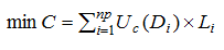 |
(1) |
Where C=total cost (monetary units problem dependant); np=number of pipes; Uc=unit pipe cost depending on the diameter selected in a specific problem; Di=diameter of pipe i; Li=length of pipe i.
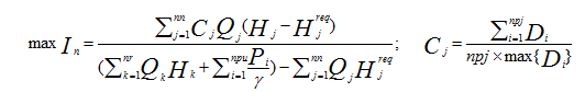 |
(2) |
Where In=network resilience; nn=number of demand nodes; Cj, Qj, Hj and Hjreq=uniformity, demand, actual head and minimum head of node j; nr=number of reservoirs; Qk and Hk=discharge and actual head of reservoir k; npu=number of pumps; Pi=power of pump i if any; γ=specific weight of water; npj=number of pipes connected to node j; Di=diameter of pipe i connected to demand node j.
MOEAs Used
NSGA-II features a fast non-dominated sorting approach, implicit elitist selection method based on Pareto-dominance rank and a secondary selection method based on crowding distance, which significantly improve its performance on difficult multi-objective problems. Moreover, it provides a constraint-handling technique to deal with constrained problems efficiently and supports both binary and real coding representations. More details about NSGA-II readers are referred to the following paper:
- Deb, K., Pratap, A., Agarwal, S., Meyarivan, T., 2002. A Fast and Elitist Multiobjective Genetic Algorithm: NSGA-II. IEEE T. Evolut. Comput. 6(2), 182-197.
The source code of NSGA-II was written in C and can be downloaded from the KanGAL website.
AMALGAM is a hybrid optimisation framework which employs four sub-algorithms simultaneously within its structure, including NSGA-II, adaptive metropolis search, particle swarm optimisation and differential evolution. It is designed to overcome the drawbacks of using an individual algorithm. The strategies of global information sharing and genetically adaptive offspring creation are implemented in the process of population evolution. Each sub-algorithm is allowed to produce a specific number of offspring based on the survival history of its solutions in the previous generation. The pool of current best solutions is shared among sub-algorithms for reproduction.
More details about AMALGAM readers are referred to the following paper:
- Vrugt, J. A., Robinson, B. A., 2007. Improved Evolutionary Optimization from Genetically Adaptive Multimethod Search. Proc. Natl. Acad. Sci. U.S.A. 104(3), 708-711.
The source code of AMALGAM was written in Matlab and can be obtained by request on their website.
Unlike the NSGA-II, ε-MOEA is a steady-state MOEA in which only one solution is generated per iteration. It incorporates the concept of ε-dominance, being able to preserve a good representation of Pareto front in terms of convergence and diversity. At the beginning, a population is initialised randomly and the non-dominated solutions are retained in an archive. Next, a solution is created via crossover and mutation using two parents each of which selected from the population and the archive. Then, this solution is checked for acceptance or rejection by the population and the archive, using Pareto dominance and ε-dominance, respectively. The abovementioned procedure is repeated until a stopping criterion is met.
More details about ε-MOEA readers are referred to the following paper:
- Deb, K., Mohan, M., Mishra, S., 2005. Evaluating the epsilon-domination based multi-objective evolutionary algorithm for a quick computation of Pareto-optimal solutions. Evolut. Comput. 13(4), 501-525.
The source code of ε-MOEA was written in C and can be downloaded from the KanGal website.
Based on the steady-state structure of ε-MOEA, Borg incorporates more advanced features into a unified framework, including ε-dominance, ε-progress (a measure of convergence speed), randomised restart, and auto-adaptive multi-operator recombination (similar to AMALGAM). The advantages of Borg are threefold: (1) usage of ε-box dominance archive contributes to maintaining the convergence and diversity concurrently throughout the search; (2) the combination of time continuation, adaptive population sizing, and two types of randomised restart (i.e. ε-progress triggered restart and population-to-archive ratio triggered restart) boosts the algorithm towards global optima; (3) simultaneous employment of multiple recombination operators enhances performance on a wide assortment of problem domains. In addition, the adoption of the steady-state, elitist model of ε-MOEA make it easily extendable for use on parallel architectures.
More details about Borg readers are referred to the following paper:
- Hadka, D., Reed, P., 2013. Borg: An Auto-Adaptive Many-Objective Evolutionary Computing Framework. Evolut. Comput. 21(2), 231-259.
The source code of Borg was written in C and can be obtained by request from the BorgMOEA website.
The ε-NSGA-II method goes beyond the common implementation of MOEA by building on NSGA-II and three key components, namely ε-dominance archiving, adaptive population sizing with archive injection, and automatic termination. The ε-NSGA-II differs from the NSGA-II primarily in two aspects: (1) while the population evolves in the same manner as NSGA-II, an offline archive is frequently updated by selecting the ε-non-dominated solutions from the elitist population at current generation; (2) the optimisation is implemented in consecutive epochs, each of which is terminated automatically according to the user-specified improvement criteria. The next epoch is populated by injecting the members in the archive and generating new random solutions. The ε-dominance archiving maintains the convergence and diversity of the archive concurrently. It also allows users to specify the precision of each objective and thus is more flexible in practice. Adaptive population sizing contributes to balancing the exploration and exploitation throughout the search, which is achieved by increasing or decreasing the capacity of the population based on the number of members in the archive. Additionally, several connected runs, known as time continuation, enhance the possibility to explore other regions of search space.
More details about ε-NSGA-II readers are referred to the following paper.
- Kollat, J. B., Reed, P. M., 2006. Comparing state-of-the-art evolutionary multi-objective algorithms for long-term groundwater monitoring design. Adv. Water Resour. 29(6), 792-807.
The source code of ε-NSGA-II was written in C and can be obtained by sending the request to the authors.
Small problems
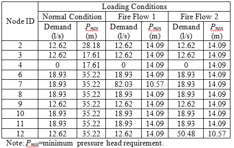
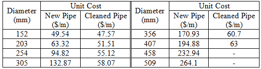
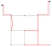
TRN has eight undetermined pipes and nine prefixed pipes, two reservoirs fixed at 365.76 m (left) and 371.86 m (right) and nine demand nodes. New and cleaned pipes have the same Hazen-Williams roughness coefficient of 120. The minimum pressure of all the nodes under three demand patterns is specified in Table TRN.1. The decision variables are the pipe diameters for five new pipes and alternative options (duplication or cleaning or leaving alone) for three existing pipes. Each pipe has eight diameter options to choose from. Table TRN.2 shows available options for pipe diameter and the corresponding unit costs. Figure TRN.1 depicts the layout of TRN.
|
Table TRN.1. Minimum pressure requirement of each node under three demand patterns of TRN |
|
|
|
Table TRN.2. Diameter options and associated unit costs of TRN |
|
|
|
Figure TRN.1. Layout of Two Reservoir Network (Undetermined pipes are shown in red lines.) |
|
|
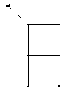
Two loop network (TLN) consists of one reservoir, six demand nodes and eight pipes organised in two loops. The reservoir has a constant head fixed at 210 m. As a hypothetical network, all pipes have the same length (1000 m) and the Hazen-Williams coefficient of 130. The pressure is set to be at least 30.0 m at all demand nodes. Table TLN.1 shows commercially available diameters and the corresponding unit costs (1 in.=0.0254 m). Figure TLN.1 depicts the layout of TLN.
| Table TLN.1 Diameter options and associated unit costs of TLN |
 |
| Figure TLN.1. Layout of Two Loop Network |
 |
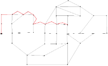
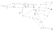
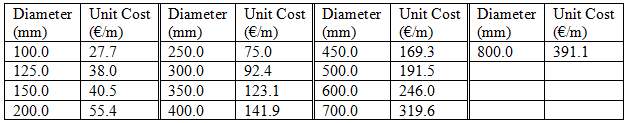
BakRyan Network (BAK) has fifty-eight pipes including nine new pipes to be sized, thirty-five demand nodes, one reservoir with a fixed head of 58 m. The Hazen-Williams roughness coefficient for each new pipe is 100. The minimum pressure head above the ground elevation of each node is 15 m. Among the new pipes, six of them are parallel. Table BAK.1 shows commercially available diameters and the corresponding unit costs. Figure BAK.1 depicts the layout of BAK.
| Table BAK.1 Diameter options and associated unit costs of BAK |
 |
| Figure BAK.1 Layout of BakRyan Network (Undetermined pipes are shown in red lines.) |
 |
Medium problems
The NYT is comprised of twenty-one pipes organised in two loops, nineteen demand nodes, and one reservoir with a fixed head of 300 ft (1 ft=0.3048 m). All the existing pipes are considered for duplication in order to meet the projected future demand. The Hazen-Williams roughness coefficient for both new and existing pipes is 100. The minimum pressure of all demand nodes is fixed at 255 ft except for node 16 and 17 that are 260 ft and 272.8 ft, respectively. A selection of fifteen diameter sizes are available as well as a ‘do nothing’ option. Table NYT.1 shows the diameter options and associated unit costs. Figure NYT.1 depicts the layout of NYT.
|
Table NYT.1. Diameter options and associated unit costs of NYT |
|
|
|
Figure NYT.1. Layout of NYT (Undetermined pipes are shown in red lines.) |
|
|
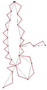
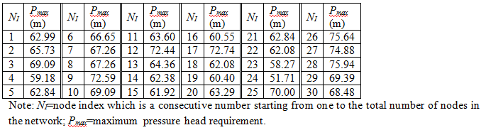
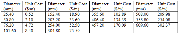
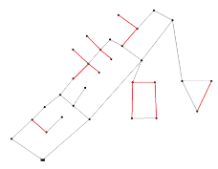
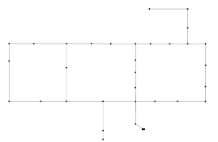
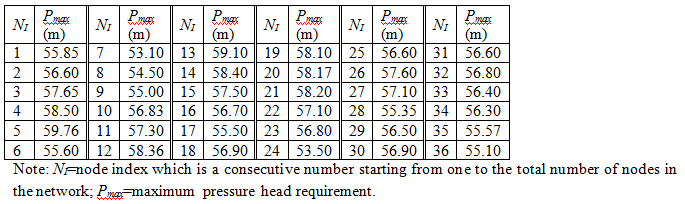
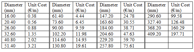
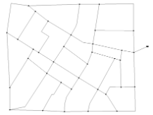
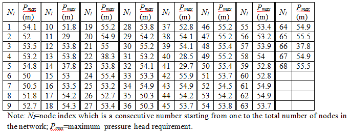
Blacksburg Network (BLA) consists of thirty-five pipes of which twelve have fixed diameters, one reservoir with a fixed head of 715.56 m, and thirty demand nodes. A universal Hazen-Williams coefficient of 120 is applied to all the pipes under consideration. The pressure requirement of each node is limited within a specified range under the single loading condition. The minimum pressure head for each node is 30 m, while the maximum pressure head varies from node to node and is provided in Table BLA.1. Table BLA.2 shows commercially available diameters and the corresponding unit costs. Figure 5 depicts the layout of BLA.
|
Table BLA.1. Maximum pressure head requirement of each node of BLA |
|
|
|
Table BLA.2. Diameter options and associated unit costs of BLA |
|
|
|
Figure BLA.1. Layout of Blacksburg Network (Undetermined pipes are shown in red lines.) |
|
|
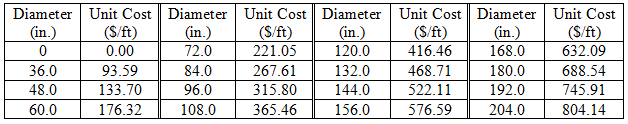
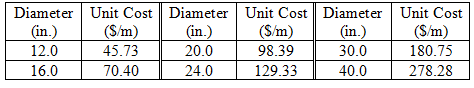
Hanoi network consists of thirty-four pipes organised in three loops, thirty-one demand nodes and one reservoir with a fixed head of 100 m. The Hazen-Williams roughness coefficient for all pipes is 130. The minimum head above the ground elevation of each node is 30 m. There are six commercially available pipe sizes, ranging from 12 in. to 40 in. (1 in.=0.0254 m). Table HAN.1 shows the diameter options and associated unit costs. Figure HAN.1 depicts the layout of HAN.
|
Table HAN.1. Diameter options and associated unit costs of HAN |
|
|
|
Figure HAN.1. Layout of HAN |
|
|
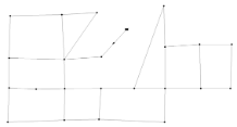
GoYang Network includes thirty pipes, twenty-two demand nodes, and one constant pump of 4.52 kW linking to one reservoir with a constant head of 71 m. The Hazen-Williams roughness coefficient for each new pipe is 100. The minimum pressure head above the ground elevation of each node is 15 m. Table GOY.1 shows commercially available diameters and the corresponding unit costs. Figure GOY.1 depicts the layout of GOY..
|
Table GOY.1. Diameter options and associated unit costs of GOY |
|
|

|
Figure GOY.1. Layout of GOY |
|
|
Intermediate problems
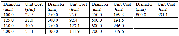
Fossolo Network (FOS) includes fifty-eight pipes, thirty-six demand nodes, and one reservoir with a fixed head of 121.00 m. The material for all the pipes is polyethylene. Due to the feature of polyethylene, a relatively high roughness coefficient of 150 is applied to all the pipes. The minimum pressure head of all the demand nodes is maintained at 40 m, while the maximum pressure head of each node is specified in Table FOS.1. In addition, the flow velocity in each pipe is enforced to be less than or equal to 1 m/s. Table FOS.2 shows commercially available diameters and the corresponding unit costs. Figure FOS.1 depicts the layout of FOS.
|
Table FOS.1. Maximum pressure head requirement of each node of FOS |
|
|
|
Table FOS.2. Diameter options and associated unit costs of FOS |
|
|
|
Figure FOS.1. Layout of Fossolo Network |
|
|
Pescara Network (PES) includes ninety-nine pipes, sixty-eight demand nodes, and three reservoirs with fixed head within 53.08 m to 57.00 m. The pipe material is cast iron. A uniform Hazen-Williams roughness coefficient of 130 is applied to all pipes. The minimum pressure head of all the demand nodes is maintained at 20 m, while the maximum pressure head of each node is specified in Table PES.1. In addition, the flow velocity in each pipe is enforced to be less than or equal to 2 m/s. Table PES.2 shows commercially available diameters and the corresponding unit costs. Figure PES.1 depicts the layout of PES.
|
Table PES.1. Maximum pressure head requirement of each node of PES |
|
|
|
Table PES.2. Diameter options and associated unit costs of PES |
|
|
|
Figure PES.1. Layout of Pescara Network |
|
|
Large problems
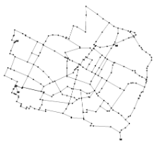
Modena Network (MOD) includes three hundred and seventeen pipes, two hundred and sixty-eight demand nodes, and four reservoirs with fixed head within 72.0 m to 74.5 m. The pipe material is the same as PES. A uniform Hazen-Williams roughness coefficient of 130 is applied to all pipes. The minimum pressure head of all the demand nodes is maintained at 20 m. The maximum pressure head of each node of MOD is provided in Table MOD.1 In addition, the flow velocity in each pipe is enforced to be less than or equal to 2 m/s. Table MOD.2 shows commercially available diameters and the corresponding unit costs. Figure MOD.1 depicts the layout of MOD.
|
Table MOD.1. Maximum pressure head requirement of each node of MOD |
|
|
MOD Table 1 Table available in Microsoft Word 2003 format due to its large size |
|
|
Table MOD.2. Diameter options and associated unit costs of MOD |
|
|
|
Figure MOD.1. Layout of Modena Network |
|
|
Balerma Irrigation Network (BIN) includes four hundred and fifty-four relatively small length pipes, four hundred and forty-three demand nodes (hydrants), and four reservoirs with fixed heads within 112 m to 127 m. The material of pipes is polyvinyl chloride (PVC). The Darcy-Weisbach roughness coefficient of 0.0025 mm is applied to all the pipes. The minimum pressure head above ground elevation is 20 m for all the demand nodes. Table BIN.1 shows commercially available diameters and the corresponding unit costs. Figure BIN.1 depicts the layout of BIN.
| Table BIN.1 Diameter options and associated unit costs of BIN |
 |
| Figure BIN.1. Layout of Balerma Irrigation Network |
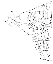 |
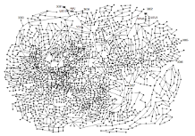
Exeter network has three thousand and thirty-two pipes including five hundred and sixty-seven considered for duplication, five valves, one thousand eight hundred and ninety-one junction nodes and seven water sources. Two major reservoirs (node 3001 and 3002) supply water to the system at fixed head of 58.4 m and 62.4 m respectively. The system is also fed by its neighbour systems via node 3003 to 3007 at fixed rates. Three non-return valves (also known as check valves) are connected to node 3001 and 3002 to control the flow direction into and outside the system. One pressure reducing valve locates in the downstream of node 3004 to maintain the downstream pressure within 58.4 m. One throttle control valve is also in the link downstream of node 3004 to control the flow and pressure of system.
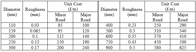
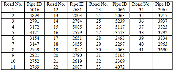
The minimum pressure requirement of demand nodes is 20.0 m. There are ten available discrete pipe sizes and one extra option as 'do nothing'. The unit cost for duplicating the existing pipe depends on both the diameter selected and the road type. Table EXN.1 shows the pipe diameters, the corresponding Colebrook-White friction factors (following Darcy-Weisbach formula) and unit costs. The location of major roads is specified in Table EXN.2 in terms of pipe ID. Figure EXN.1 depicts the layout of EXN.
|
Table EXN.1. Roughness coefficients and unit costs of EXN |
|
|
|
|
|
Table EXN.2. Location of major road in terms of pipe ID |
|
|
|
Figure EXN.1. Layout of Exeter Network1 |
|
|
1 This network is a bit different from the one available at . The modifications are summarised as follows: (1) Node 1610 has been removed to avoid isolated junction; (2) 20 PM in the section of “TIMES” of input file has been changed to 8 PM; (3) Since it is impossible for junction 1107 to meet the minimum pressure requirement, it is ignored in the calculation of constraint violation. Also, it would be too complicated to highlight all the pipes considered for duplication, these pipes are tagged in the input file given.
Data files
The following data files are available:
- True and best known Pareto Front data files;
- True and best known Pareto Front figures;
- EPANET input files;
- Source code required to run and evaluate objective functions.
True and Best Known Pareto Front Data Files
The pareto front files are available as text files where the first column represents the values of the resilience objective and the second column represents the values of the cost objective. The figures are available in Windows metafile (EMF) format.
| Type | Problem PF | Figures | EPANET Input Files |
|---|---|---|---|
| SP | Two-reservoir Network | TRN | TRN |
| Two-loop Network | TLN | TLN | |
| BakRyan Network | BAK | BAK | |
| MP | New York Tunnel Network | NYT | NYT |
| Blacksburg Network | BLA | BLA | |
| Hanoi Network | HAN | HAN | |
| GoYang Network | GOY | GOY | |
| IP | Fossolo Network | FOS | FOS |
| Pescara Network | PES | PES | |
| LP | Modena Network | MOD | MOD |
| Balerma Irrigation Network | BIN | BIN | |
| Exeter Network | EXN | EXN |
Source code
The source files are available as a single ZIP archive. This archive also contains the code and instructions on how to run the test cases using MATLAB.
Publication
Detailed description of the optimisation methods used to generate the data are given in the publication:
References
- [1] Gessler, J., 1985. Pipe network optimization by enumeration, In Proc., Computer Applications for Water Resources. ASCE: New York, N.Y., pp. 572-581.
- [2] Alperovits, E., Shamir, U., 1977. Design of optimal water distribution systems. Water Resour. Res. 13(6), 885-900.
- [3] Lee, S.C., Lee, S.I., 2001. Genetic algorithms for optimal augmentation of water distribution networks. J. Korean Water Resour. Assoc. 34(5), 567-575.
- [4] Schaake, J., Lai, D., 1969. Linear programming and dynamic programming application to water distribution network design, Dept. of Civil Engineering, Massachusetts Institute of Technology, Cambridge, Massachusetts.
- [5] Sherali, H., Subramanian, S., and Loganathan, G. V. 2001. Effective relaxations and partitioning schemes for solving water distribution network design problems to global optimality. J. Global Optim., 19(1), 1–26.
- [6] Fujiwara, O., Khang, D., 1990. A two-phase decomposition method for optimal design of looped water distribution networks. Water Resour. Res. 26(4), 539-549.
- [7] Kim, J.H., Kim, T.G., Kim, J.H., Yoon, Y.N., 1994. A study on the pipe network system design using non-linear programming. J. Korean Water Resour. Assoc. 27(4), 59-67.
- [8] Bragalli, C., D'Ambrosio, C., Lee, J., Lodi, A., Toth, P., 2012. On the Optimal Design of Water Distribution Networks: a Practical MINLP Approach. Optim. Eng. 13, 219-246.
- [9] Reca, J., Martínez, J., 2006. Genetic algorithms for the design of looped irrigation water distribution networks. Water Resour. Res. 42(5), W05416.
- [10] Farmani, R., Savic, D.A., Walters, G.A., 2004. "EXNET" Benchmark Problem for Multi-Objective Optimization of Large Water Systems, Modelling and Control for Participatory Planning and Managing Water Systems, IFAC workshop: Venice, Italy.